![]()
PMM-Lab is an open-source extension to the Konstanz Information Miner (KNIME). It consists of three components:
- a library of KNIME nodes (called PMM-Lab),
- a library of “standard” workflows
- a HSQL database to store experimental data and microbial models.
Altogether these components are designed to ease and standardize the statistical analysis of experimental microbial data and the development of predictive microbial models (PMM). Users can apply PMM-Lab to proprietary or public data and create bacterial growth / survival / inactivation models. The framework can easily be extended to other model types, e.g. growth/no-growth boundary models. PMM-Lab has been initiated and provided by the German Federal Institute for Risk Assessment – BfR (Berlin, Germany). The software is in Beta status. Before using the software you have to read and accept the license and disclaimer, https://sourceforge.net/p/pmmlab/wiki/Disclaimer/. If you do not agree, do not use this software.
Source code: https://github.com/SiLeBAT/PMM-Lab
Disclaimer
- All reasonable efforts have been made to ensure that PMM-Lab is provided free of errors and up to date. Anyhow, no guarantee as to the accuracy and completeness of PMM-Lab or the work resulting from PMM-Lab application or the fitness of PMM-Lab for any purpose whatsoever is given.
- PMM-Lab may change at any time without notice.
- PMM-Lab is provided ‘as is’, without any conditions, warranties or other terms of any kind.
- There is no liability for any loss or damage arising from any inability to use PMM-Lab.
- The developers and the BfR exclude all liability and responsibility for any amount or kind of loss and damage that may result to you or a third party (including without limitation, any direct, indirect, punitive or consequential loss or damages), or loss of income, profits, goodwill, time, data, contracts, use of money, or loss or damages from or connected in any way to business interruption – including but not limited to loss or damage due to viruses that may infect your computer equipment, software, data or other property on account of your use of PMM-Lab or your downloading of any material from PMM-Lab or any web site linked to PMM-Lab.
PMM-Lab tutorial
PMM-Lab is an extension of the Konstanz Information Miner (KNIME). For getting started, you may want to make yourself familiar with this software product. Documentation can be obtained from http://tech.knime.org/documentation.
Nevertheless for this introduction no prior knowledge on KNIME is required. In this section we will give you a short introduction to the Scientific Workflow concept and KNIME. Furthermore, we will give an introducing example for the application of PMM-Lab to predictive microbiology.
The concept of Scientfic Workflows
KNIME is a Scientific Workflow Management system. A Scientific Workflow consists of interconnected task nodes. Each task node is responsible for a specific data processing step. The connections between task nodes describe the data dependencies between the tasks. Such tasks may be the data loading, storing or manipulation. After describing all necessary data processing task in a so called workflow, this workflow can be executed and the calculations will be performed in a transparent and repeatable fassion. The same concept is applied in PMM-Lab where workflows serve as an easy to understand user interface to the dataprocessing steps which can easily adapted by the user to its specific needs. The graphical description of data processing steps is usually considered as an intuitive way to increase transparency within data analysis and modeling tasks.
Organization of the KNIME user interface
The KNIME graphical user interface divides the screen into a set of different compartments (views). For us, the most important views are:
- Workspace (KNIME_project)
- Node Repository
- Console
- Node Description
- Workflow Projects
When starting up KNIME, an empty workspace is shown. In the workspace we can assemble a workflow out of nodes and connecting arrows that represents the data flow and, hence, the Scientific Workflow. In the node repository view, all task nodes are listed that can be utilized in a workflow. KNIME comes with a set of standard nodes libraries. PMM-Lab is essentially a new extension to this node repository. After installing the PMM-Lab plugin, a new node library folder called ‘PMM-lab’ can be found in the node repository. The Console view prints out messages, warnings and errors that are produced by configuring or executing the workflow. Eventually, in the Node Description view gives information on the functionality and configuration options of each node. The Workflow Projects view shows all workflows in the current workspace. It is possible to organize workflows in folders and to rename, copy or move them.
Setting up an example workflow
We will now set up a simple workflow for the purpose of introducing the basic operations that can be performed with PMM-Lab. We will go through the assembly of the Workflow step by step and explain the way each node works and how these are interconnected in a meaningful way. If you want an overview about the functionality that PMM-Lab provides, please refer to the feature description section. If you want to explore the available KNIME nodes and what they can do, please go to the node description section. The first thing we will have to accomplish is to create a new KNIME workflow.
- ‘File’
- ‘New…’ the ‘Select a wizard’ window opens.
- Select ‘New KNIME Workflow’ from the ‘Wizards:’ list.
- Click the button ‘Next >’
- You may enter a custom workflow name in the text field ‘Name of the workflow to create:’
- Click the button ‘Finish’
An empty KNIME workflow tab will open. Note that the new workflow appears in the ‘Workflow Projects’ window where you can organize all workflows you created. In our example workflow we will create primary growth models from data sets. After the creation of the model we will visualize the result and save the models to the PMM-Lab database.
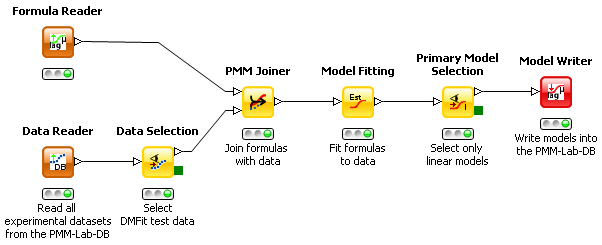
This workflow demonstrates how to fit primary models to experimental microbial data.
- Read in microbial data to work with (e.g. with ComBase Reader, Data Reader etc.). If necessary you can visualize and select data by applying the Data Selection node – in this case we select all DMFit test data.
- Select the model formulas which should be fitted to the data by configuring the Formula Reader node. In the example below the full Baranyi growth model (iPMP model eq. 6), the Huang model (iPMP model eq.5) and the three-phase linear model (iPMP model eq. 8) are selected. Equally well a formula would work that a user enters in the Formula Creator node or in the Model Creator node. Attention: the Creator nodes give you also the opportunity to assign units to the variables!
- Connect the Formula Reader and Data Selection node out-ports with the in-ports of the PMM Joiner node and then configure the PMM Joiner node. To do the latter either double-click the node, right-click and choose ‘Configure…’ or press F6 on the keyboard. In the configuration menu you need to assign the correct columns from the data table to the independent / dependent variables of the formula(s). Then the PMM Joiner node can be executed. Attention: based on the unit of the dependent variable the experimental data will be transformed by this node, e.g. if the formula expects ln()-scaled values the log10()-scaled measured data will be transformed automatically. If you do not want that you have to provide a formula with a log10()-scaled dependent variable.
- Execute the Model Fitting node. In case the standard setting does not provide a sufficiently good fitting result, tick ‘Expert settings’ and providing starting values for any of the model parameters. Fitting itself may take a while, depending on the number of models and data sets to be fitted.
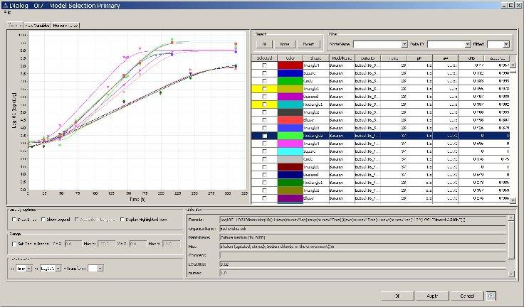
- Look at the model fitting results by application of the Primary Model Selection node. This node allows the manual selection / deselection of models according to your personal criteria (e.g. RMS, RSquare, model type etc.). In the node GUI you can also configure which columns in the tabular listing of fitted models should be on display. Attention: SSE, RMSE, MSE are scaled to the log-transformation defined by the selected formula. Only RSquared can be used to compare models with different log-transformation directly. This node also provides the opportunity to select models for further processing – in the example below all models fitted to the three-phase linear formular (iPMP eq. 8) are selected. After execution, the green outport of the Primary Model Selection node contains the graph as PNG image.
- Depending on the individual preference you can save the selected models to the PMM-Lab database or write them to a KNIME data table (Table Writer). In case of the first option you could verify that the models have been written correctly with all relevant parameters into the DB table “Estimated models” via the Menu item “PMM-Lab -> Open DB GUI …” . The Model Reader node enables the user to retrieve the models back from the PMM-DB.
PMM-Lab resources
Sample workflows
When the installation of PMM-Lab is finished we suggest to start working with the program by downloading our sample workflows for primary and secondary model estimation.
After downloading you can import them one by one via: File -> Import Knime Workflows -> Select archive file -> browse … -> Finish;
You find the workflow in the KNIME Explorer Window under “LOCAL (Local Workspace)”. By double clicking the selected workflow will be opened and you can execute / modify / play with it.
If you would like to extend these workflows you can use all nodes from the node library in the Node Repository. There also the PMM-Lab node repository is located.
Microbiological data for model fitting
A popular online resource for microbial data is the ComBase. It comprises a plethora of growth and inactivation data and PMM-Lab provides a compatibility layer that lets you import and export files formatted in the way they are offered by ComBase. The ‘ComBase Reader’ and the ‘ComBase Writer’ nodes accomplish these tasks.
In scientific literature results of microbial growth, survival or inactivation experiments are described heterogeneously in different units. In some cases it is impossible to transform this data to a more standardized unit lateron, like e.g. log10(CFU/g) or log10(CFU/ml). In PMM-Lab the data model defines cell concentration the way that the cell/virus concentration is represented in log10(cells/CFU/units/vp/pfu per g) or log10(cells/CFU/units/vp/pfu per ml) (decadic logarithm). Time is always represented in hours.
This treatment of units has been selected to be consistent with the data handling in the ComBase as documented in a Tutorial for submitting data to ComBase.
Formula notation
PMM-Lab comes with a number of preset formulas that you can deploy right away. You may, however, want to create your own models. The node “Model Creator” gives you the possibility to create and edit model formulas inside PMM-Lab. For these formulas PMM-Lab uses infix notation and a number of common math functions are available. You may use
sqrt(x) to calculate the square root of the expression x … An important part of PMM-Lab formula notation is the disambiguation of the logarithm function. In contrast to other programming languages, in PMM-Lab, the function log(x) refers to the decadic logarithm. To avoid ambituity among the various logarithm functions, you may prefer to use the functions ln(x) for the natural logarithm with base e and log10(x) to refer to the decadic logarithm.
In your formulas you can also use conditional operators. For example
t<=1
evaluates 1 if t is smaller or equals 1 whereas it evaluates 0 otherwise. You may use the following operators accordingly:
| < | > | <= | >= | && | || |
Initialization range of formula parameters For each parameter in a formula you can impose an initialization range. This range will be used for initializing the algorithm that tries to find the optimal parameter set. It is not mandatory that the actual parameters lie within this range. You will, however, be notified if estimated parameters lie outside their initial definition range.
Curve fitting
Curve fitting is a central aspect of PMM-Lab. In this section we will present, in what kind of use cases you may want to fit a curve and how to accomplish that. Furthermore, we will introduce, how the fitted models can be further processed and how to visualize the obtained results.
Use cases
There are two distinct scenarios in which you might want to fit a curve.
- Given a microbial data set, you want to derive a model that approximates the tenacity behavior under just the same conditions that gave rise to this data set.
- Given the model parameters derived under a variety of conditions, you want to derive a model that approximates the value of the model parameters dependent on these conditions.
While the first scenario describes the estimation of a Primary Model, the latter scenario represents a Secondary Model. We will refer to these two concepts quite frequently. Hence, its understanding is paramount for the upcoming discussion.
Primary Model Fitting
In Primary Model Fitting, we consider bacterial growth or inactivation as the concentration of a bacterial agent dependent on the time. So
t -> log10(C)
In PMM-Lab this mapping is implemented as a function dependent on a set of parameters p. Hence,
| log10(C)=f(t | p) |
It is the goal of the Fitting process to derive a realization of the parameter set p that approximates a given data set D as accurately as possible. Consequently, the fitting of a Primary Model consumes a microbial data set D and outputs a set of parameters p, the primary model.
Seconday Model Fitting
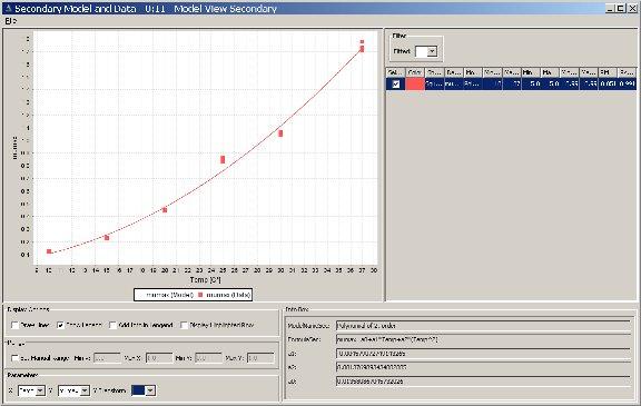
In Secondary Model Fitting, we assume that bacterial kinetics depend on the environmental conditions e under which the original experiment has been conducted. So
e -> p In PMM-Lab, a model that implements this mapping also depends on a set of parameters s. Hence,
| p=f(e | s) |
So, in Secondary Model Fitting we try to find a parameter set s that approximates the parameters for a primary model as accurately as possible for given environmental conditions. Consequently Secondary Model Fitting consumes examples of environmental conditions e and the primary model parameters p associated to them, and produces a set of secondary parameters s.
Curve fitting in PMM-Lab In PMM-Lab, both Primary and Secondary Model Fitting are performed by a single KNIME node called “Model Fitting”. The node knows, when to perform what from the KNIME table presented to it. If given a combination of a Microbial Data Set and a Primary Model Formulas, it performs a Primary Model fit. If presented a combination of fitted Primary Models and Secondary Models, if performs a Secondary model fit.
Model selection
In PMM-Lab, it is possible to fit several models to the same data set. The advantage of this approach is the fact that one can choose the most appropriate model for the data set at hand. Models differ in their theoretical foundation, complexity, their robustness and their ease of interpretation. It is the researcher’s responsibility to choose the model as a compromise according to the aforementioned aspects. This task is generally referred to as model selection.
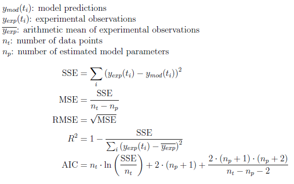
PMM-Lab provides several measures with which the researcher can quantify the performance of his model.
- Root Mean Square (RMS)
- Statistic coefficient of determination R2
- Akaike Information Criterion (AIC)
The former two measures only quantify the error with respect to the training data set. The latter as well considers model complexity. I.e. simple models are preferred in favor of complex ones.
Root Mean Square
The Root Mean Square (RMS) error is a measure for the difference between a data set and a corresponding fit. The RMS asymptotically converges to the standard deviation from the model’s predicted value for sufficiently large sizes of data sets.
Statistic coefficient of determination
The R2 value or statistical coefficient of determination is a measure for how well a regression model is capable of describing a data set. The R2 does not explicitly consider model complexity. Its definintion range is (-inf,1]. Where 1 is a perfect fit while 0 is equivalent to the fit of an uninformed model that plainly predicts the expectation value of the dependent variable and is ignorant with respect to the independent variables. Hence, a model, that performs with an R2 < 0 is expected to lose information on observation of the set of dependent variables instead of gaining. This situation is, of course, undesirable.
Akaike Information Criterion
Similarly to the BIC, the Akaike Information Criterion (AIC) describes the goodness of fit for a model with respect to model complexity. Penalty for complexity in the AIC is less severe than in BIC, thereby emphasizing accuracy over simplicity in comparison with the BIC.
Formulas
Formulas used in PMM-Lab: